Example of applying a profile to a worksheet
An example of applying a profile, based on an Uplift trend, to a worksheet. When you access a worksheet, with a shared scenario, and select the option, this process is implemented:
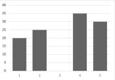
The applicable data:
- Profile sequence = 20, 25, 0, 35, 30.
- Start Period = FY14 M08.
- Uplift = 100.
- Downturn = 0 (disabled, as there are no negative data points for the profile).
- Net = 100.
The specified Uplift, or Downturn, or both the values are applied from the start period to the 5 adjacent cells on the right, based on the number of values specified in the profile. For example, the FY14 M08, FY14 M09, FY14 M10, FY14 M11, and FY14 M12 periods are the top dimension periods that display the months. Also, each cell is allotted an equal proportion of the net change, based on the profile ratios.
If a profile point is linked to a positive value, the value applied to the cell is:
Uplift * (profile data value / profile total positive values).
If a profile data point is linked to a negative value, the value applied to the cell is:
[Downturn * (profile data value / profile total negative values)] * - 1.
As a result:
- FY14 M08 = 100 * (20 / 110) = 18
- FY14 M09 = 100 * (25 / 110) = 23
- FY14 M10 = 100 * (0 / 110) = 0
- FY14 M11 = 100 * (35 / 110) = 32
- FY14 M12 = 100 * (30 / 110) = 27