Holt-Winters Multiplicative trend and seasonality method
This method takes both trend and seasonality into consideration. A seasonal index is added to the equation.
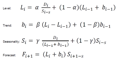
Where s is the seasonality period length.
For 0 ≤ α ≤ 1, 0 ≤ β ≤ 1 and 0 ≤ γ ≤ 1.
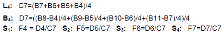
To get started, initial values of the level, trend and seasonality are required. To
initialize the seasonality, a minimum of one complete seasonal cycle is required  .
.
The initial values for  are calculated based on:
This table displays the initializations for Holt-Winters 4 Multiplicative:
Note: For initialization, L(4) is used to set up seasons S(1) to S(4). The
end calculation point is Period 25, which is the period immediately after the last demand.
Initialization depends solely on the seasonality range, not on alpha, beta, or gamma.
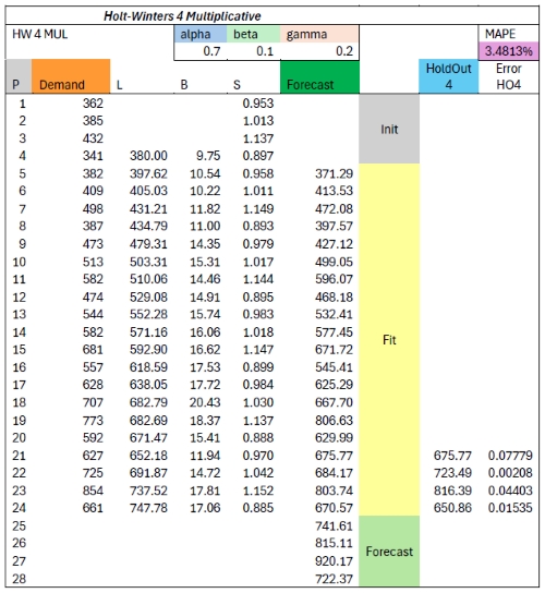
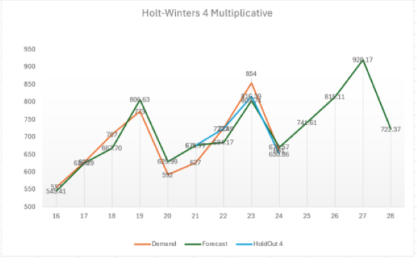
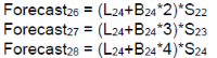
Extrapolation of Holt-Winter
For extrapolation, the last season range is repeated and Trending (B in period 24) is added.
On , the forecast is calculated with m=1.
In Forecast Method Properties, select . Specify the values in each these fields:
- Smoothing constant - Alpha determines how fast the algorithm adapts to leveling and to some degree this leveling influence seasonality as well.
- Smoothing constant - Beta determines how fast the algorithm adapts to trending.
- Smoothing constant - Gamma determines how fast the algorithm adapts to seasonality.
Lower gamma allows the algorithm to remember more strongly:
- Gamma = 0 means only the initial seasonality is used.
- Gamma = 1 means only the latest period range is used.