To create distribution histograms
Distribution Histograms are used to ascertain the variation by displaying a standard distribution curve of measured values for an item.
To plot this chart you must select the combination of item or item/supplier, inspection order source, aspect/characteristic as well as the relevant time period. This chart is based only on actual inspection results.
The centre line of the distribution curve is the LN calculated mean (µ). The over/under tolerance limits of the process are the limits within which the process is capable of producing parts of an acceptable quality. These tolerance limits are generally expressed as the process mean plus or minus 3 standard deviations (σ) that can capture 95 percent of the normal variance spread.
To plot this type of chart, complete the following steps:
- Calculate measured values for a range of periods.
- Determine the spread R of the measured values: R = Xmax – Xmin
- Determine the class width: W = R / SQRT (number of measurements)
- Compose the classed: Class 1 Lower Tolerance (or Xmin in case Xmin < Lower Tolerance) then Class2 = Class1 + W and so on
- Populate the classes based on the measured values. Determine the frequency within each class.
- Calculate the arithmetic means of the measured values.
- Calculate the standard deviation
- Plot the histogram based on the classes calculated.
Example
Assume that 5 inspection orders are processed, each with 1 sample, resulting in one sample group for each order. All 5 inspection orders have a sample size of 10 pieces and a test quantity of 1 piece. The following results are displayed in the test data table:
| Sample Group | Sample Number | Measured Value |
| 1 | 1 | 1 |
| 1 | 2 | 1 |
| 1 | 3 | 1.002 |
| 1 | 4 | 0.997 |
| 1 | 5 | 1 |
| 1 | 6 | 1.001 |
| 1 | 7 | 1 |
| 1 | 8 | 1 |
| 1 | 9 | 1 |
| 1 | 10 | 0.999 |
| 2 | 1 | 1 |
| 2 | 2 | 0 |
| 2 | 3 | 0 |
| 2 | 4 | 0 |
| 2 | 5 | 0 |
| 2 | 6 | 0 |
| 2 | 7 | 0 |
| 2 | 8 | 0 |
| 2 | 9 | 0 |
| 2 | 10 | 0 |
| 3 | 1 | 1.001 |
| 3 | 2 | 1 |
| 3 | 3 | 0.9 |
| 3 | 4 | 0.988 |
| 3 | 5 | 1.001 |
| 3 | 6 | 1.004 |
| 3 | 7 | 0.999 |
| 3 | 8 | 0.989 |
| 3 | 9 | 1.012 |
| 3 | 10 | 1.03 |
| 4 | 1 | 1.001 |
| 4 | 2 | 1 |
| 4 | 3 | 0.9 |
| 4 | 4 | 0.988 |
| 4 | 5 | 1.001 |
| 4 | 6 | 1.004 |
| 4 | 7 | 0.999 |
| 4 | 8 | 0.989 |
| 4 | 9 | 1.012 |
| 4 | 10 | 1.03 |
| 5 | 1 | 1.001 |
| 5 | 2 | 1 |
| 5 | 3 | 0.9 |
| 5 | 4 | 0.988 |
| 5 | 5 | 1.001 |
| 5 | 6 | 1.004 |
| 5 | 7 | 0.999 |
| 5 | 8 | 0.989 |
| 5 | 9 | 1.012 |
| 5 | 10 | 1.03 |
Calculate the spread
Determine the spread of the measured values. The highest measured value is 1.03 (Sample Group 1, Sample Number 10). The lowest measured value is 0.9 (Sample Group 1, Sample Number 3).
Spread = 1.03 - 0.9 = 0.13Calculate the class width:

The class width is 0.13 / √50 = 0.02055480479109446565799280803881. This value is rounded off to 0.02.
Compose the classes
The classes are composed as follows Class 1 Lower Tolerance (or Xmin in case Xmin < Lower Tolerance) then Class2 = Class1 + W and so on. The following classes are generated:
| Class 1 | 0.900000 |
| Class 2 | 0.920000 |
| Class 3 | 0.940000 |
| Class 4 | 0.960000 |
| Class 5 | 0.980000 |
| Class 6 | 1.000000 |
| Class 7 | 1.020000 |
Populate the classes
The values of the different measurements can be grouped into a class, if the value is greater or equal to the class value, and less than the class value + the class width. The result is:
| Class | Number of measurements |
| 1 | 1 |
| 2 | 0 |
| 3 | 0 |
| 4 | 0 |
| 5 | 12 |
| 6 | 36 |
| 7 | 1 |
Calculate the mean
For every measurement, the difference to the mean is calculated and the square of the differences is added together. If the first sample number has a measurement value of 1:
(1 - 0.995850)² = (0.00415)² = 0.0000172225The square of the differences are calculated and summed together to form a total square difference. For the above example the total is 1.311734.
Mean = Standard Deviation - √ 1.311734 /
		  50 = 0.160000
Plot the chart
The following figure displays the chart plotted with the above data:
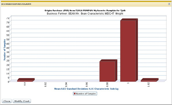
On the X-Axis the characteristics unit is displayed. It is however possible that for a specific standard test procedure or for an inspection order line, the measurement value is expressed in a different unit that are later converted to the characteristic unit.