Forecast method: polynomial regression
The relevant parameters for this forecast method are:
- Degree for Polynomial Regression
- Type of Seasonal Influence
- Seasonal Cycle Time
- Automatic Update of Forecast Parameters
You can maintain these parameters in the Plan Items - Forecast Settings (cpdsp1110m000) session.
The polynom's degree is indicated by the Degree for Polynomial Regression field. If the Automatic Update of Forecast Parameters check box is selected, LN determines the polynom's optimum degree.
Trend-adjusted average demand
First, the historical demand figures are adjusted with the trend-adjusted average demand for the relevant period.
Without seasonal influence:
TD(t) = AVWith a linear trend influence:
TD(t) = CS + TF * tWith a progressive trend influence:
TD(t) = BS * TF ^ (t-1)DM(t) = AD(t) - TD(t)Where:
| DM(t) | trend-adjusted average demand for period t |
| TD(t) | trend-based demand for period t |
| AD(t) | actual demand for period t |
| AV | average demand (*) |
| CS | constant demand |
| BS | estimated demand for period 1 |
| TF | trend factor |
(*) The average demand is the sum of the historical demand figures by period, divided by the number of periods with demand history.
Coefficients of the polynom
LN calculates the coefficients of the polynom with the polynomial regression method. See the Related topics for more information about polynomial regression.
Demand forecast
LN calculates the demand for each forecast period based on the trend-adjusted average demand for the period in question, increased with the average noise in the past.
Noise
The noise is the fluctuation of the demand data compared to the trend that has been determined. The average noise is determined for each forecast period based on the history periods which are a whole number of seasonal cycles ago.
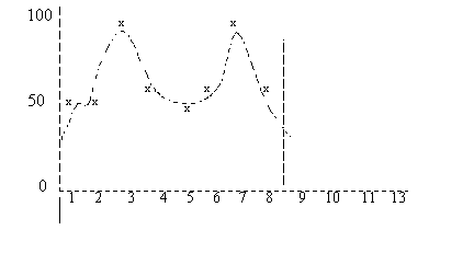
Example
This diagram shows the history demand data of two seasonal cycles, which consist of 8 forecast periods. Period 9 is the current period.

SCT = seasonal cycle time
This diagram shows the polynom that is determined with polynomial regression.
For each history period, the demand based on the polynom is compared to the trend of the demand. A linear trend is assumed to be present, characterized by the following formula:
TD(t) = CS + TF * t| TD (t) | trend based demand for period t |
| CS | constant demand (= 54) |
| TF | trend factor (= 2) |
| Period | Polynom | Trend | Noise |
|---|---|---|---|
| 1 | 45 | 56 | -11 |
| 2 | 53 | 58 | -5 |
| 3 | 76 | 60 | +16 |
| 4 | 70 | 62 | +8 |
| 5 | 49 | 64 | -15 |
| 6 | 55 | 66 | -11 |
| 7 | 78 | 68 | +10 |
| 8 | 70 | 70 | +0 |
The average noise based on these differences is added to the trend-adjusted demand. For example, the average noise for forecast period 9 is the average of the noise of periods 1 and 5.
| Forecast period | Trend | Average noise | Based on periods | Forecast demand |
|---|---|---|---|---|
| 9 | 72 | -13 | 1,5 | 59 |
| 10 | 74 | -8 | 2,6 | 66 |
| 11 | 76 | +13 | 3,7 | 89 |
| 12 | 78 | +4 | 4,8 | 82 |
| 13 | 80 | -13 | 1,4 | 67 |
| 14 | 82 | -7 | 2,6 | 75 |
This diagram shows the result:
