Allocation methods: examples
These examples show several use cases and how the various allocation options can be used to address different scenarios.
Example 1: Allocating proportionally by source
The first example shows how the amounts to be allocated are calculated and discharged proportionally by source.
In this example, 50% of the Travel Expenses (G&A) account that is not assigned to any cost center is allocated to the Marketing cost center. You can review the allocation configuration in the demo data. The corresponding allocation step is Travel Expenses G&A to Marketing. This step is assigned to Level 1.
During the allocation process, the value of the defined source area is detected, multiplied by the defined percentage, and allocated to the target. For all dimensions where no element has been defined, the total number for the dimension is allocated.
This table shows the parameterization of allocation for the corresponding allocation step:
| Parameter | Source | Target |
|---|---|---|
| Version | Budget 1 | Budget 1 |
| Allocation type |
% of data area Percent: 50% |
Proportionally by source |
| Reference dimension | Organization: Unassigned | Organization: Marketing |
| Data Area | N/A | N/A |
This diagram shows how the source data is used to calculate the values to be allocated:
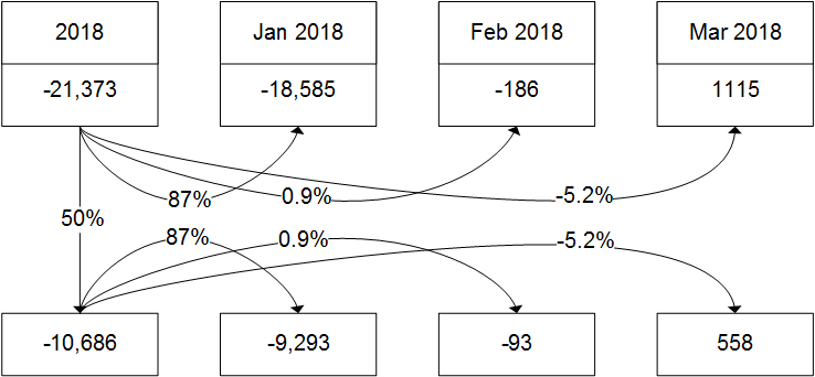
In this example, only the consolidated element, 2018, and three months January, February, and March are shown.
-21,373 x 50% = -10,686Value for month X = Total value to be allocated x Percentage for month X of the total in Source Area For January 2018, for example, the amount of Travel Expenses (G&A) account that are not assigned to any cost center is -18,585. This value represents 87% of the total amount for 2018. The value to be allocated to Marketing for January 2018 is equal to -9,293. This corresponds to the fraction of 87% of the value to be allocated for 2018, that is, -10,686.
Value for Jan = -10,686 x 87% = -9,293 Similarly, the values to be allocated are calculated for other months. For March, the value of 1,115 corresponds to -5.2% of the total for 2018. To calculate the value to be allocated for March, we must multiply the total value to be allocated with the corresponding percentage for March.
Value for Mar = -10,686 x (-5.2%) = 558 These filters are applied for the Data Flow Analysis that is used in this example:
- Configuration set: 2018-20
- Version: Budget 1
- Group: Allocation Level 0001
- Entity: Genesis Cars
- Segment 2: All Segments 2Note: Segment 2 represents the reference dimension.
- Time: 2018
- Account: Travel Expenses (G&A)
Example 2: Basis X Factor with Zero Out discharge method
In this example, to purchase materials at lower prices, a training organization buys pens and other materials in large quantities. The purchases are made a couple of times during the year. Based on the corresponding billing periods, the finance department reports these costs for specific months. The months in which these purchases are made show worse results. But results for other months in which no additional material purchases were made are better.
Controlling might use the average material costs from the previous year to calculate a cost factor, for example, a value of $2.50 per student. This factor can be used to allocate the calculated amount each month. In this example, the number of students is the driver. The amount of $2.50 per student is the Basis X Factor. By multiplying the number of students by a factor of $2.50, you can calculate the material costs for each month.
Simultaneously, the Zero Out discharge method can be used to eliminate the peaks of the original material costs provided by finance in corresponding billing months.
This table shows the results of Basis X Factor allocation and how the Zero Out option can be used:
| Month | Material Costs | Students | Calculated Costs | Zero Out | Difference |
|---|---|---|---|---|---|
| Jan | $0.00 | 1,000 | $2,500.00 | $0.00 | $2,500.00 |
| Feb | $25,000.00 | 1,100 | $2,750.00 | - $25,000.00 | - $22,250.00 |
| Mar | $100.00 | 2,200 | $5,500.00 | - $100.00 | $5,400.00 |
| Apr | $0.00 | 2,100 | $5,250.00 | $0.00 | $5,250.00 |
| May | $0.00 | 2,500 | $6,250.00 | $0.00 | $6,250.00 |
| Jun | $3,000.00 | 600 | $1,500.00 | - $3,000.00 | - $1,500.00 |
| Jul | $18,000.00 | 600 | $1,500.00 | $18,000.00 | - $16,500.00 |
| Aug | $0.00 | 0 | $0.00 | $0.00 | $0.00 |
| Sep | $0.00 | 2,100 | $5,250.00 | $0.00 | $5,250.00 |
| Oct | $1,900.00 | 3,200 | $8,000.00 | - $1,900.00 | $6,100.00 |
| Nov | $0.00 | 3,000 | $7,500.00 | $0.00 | $7,500.00 |
| Dec | $1,000.00 | 1,600 | $4,000.00 | - $1,000.00 | $3,000.00 |
| Sum | $49,000.00 | 20,000 | $50,000.00 | - $49,000.00 | $1,000.00 |
Overall, the results of February, June, and July are better when costs are distributed for all months proportionally to the number of students. The calculated costs that are based on the Basis X Factor of $2.50 might not match exactly the material costs that were reported by finance. Nevertheless, the costs are distributed more evenly across the year than based on the original material costs from finance.
Example 3: Basis X Factor allocation in the demo data
You can use this example to review how the Basis X Factor is used in the demo data and how the allocation values are calculated. The basic configuration in the demo data uses the Basis X Factor in Level 1. The corresponding allocation step is Step 3, Other Operating Expenses (Material) based on Revenues.
This table shows the Parameterization of Allocation for allocation Level 1, Step 3:
| Parameter | Source | Driver | Target |
|---|---|---|---|
| Version | Budget 1 | Budget 1 | Budget 1 |
| Allocation type | Basis X Factor | N/A | Proportionally by Target |
| Factor: 0.02 | Driver: Revenues | N/A | |
| Reference Dimension | N/A | Segment 1: Automotive | Segment 1: Automotive |
| Data Area | N/A | Segment 1: Automotive | Segment 1: Automotive |
| Segment 2: All Segments 2 | Segment 2: All Segments 2 |
This example demonstrates the allocation that is based on the revenue of the Automotive element in Segment 1. In this example, the Basis X Factor is used to charge additional costs that represent a fraction of 0.02 of the revenue. The additional costs are to be allocated to the logistic department.
In the source area, the Basis X Factor gets defined. In the driver section, the Revenue account for Automotive segment is selected. To determine the proportion of revenues across all regions, All Segments 2 element is selected.
For all other dimensions, which are not specifically defined in the parameters, the proportion of the target is used. If the target area is zero, the allocation process cannot determine the proportion and fails. Therefore, Alternate Target Configuration should be used to define how to allocate values per dimension if the specified target area is empty.
This table shows how revenue, which is defined as the driver, is distributed within Segment 2 elements. Only selected elements with non-zero values are displayed:
| Location | Revenue | Revenue % |
|---|---|---|
| All Segments 2 | 525,000,000.00 | 100.00% |
| Europe | 375,000,000.00 | 71.43% |
| Switzerland | 184,920,000.00 | 35.22% |
| Great Britain | 190,080,000.00 | 36.21% |
| Middle East | 150,000,000.00 | 28.57% |
| Jordan | 80,000,000.00 | 15.24% |
| Saudi Arabia | 70,000,000.00 | 13.33% |
For example, the revenue for the Middle East is 150,000,000. This value corresponds to 28.57% of revenues for all segments, 525,000,000.
This table shows the data allocation that corresponds to Data Flow Analysis for the selected allocation step. The selected account is Other Operating Expenses (Material). The values are allocated according to the distribution of revenues across locations that are specified in Segment 2:
| Segment 2 | Pre-Allocation | Discharged | Charged | Post-Allocation |
|---|---|---|---|---|
| All Segments 2 | -7,956,000.00 | 0.00 | -10,500,000.00 | -18,456,000.00 |
| Unassigned | -16,000.00 | 0.00 | 0.00 | -16,000.00 |
| Europe | -5,640,000.00 | 0.00 | -7,500,000.00 | -13,140,000.00 |
| Switzerland | -3,720,000.00 | 0.00 | -3,698,400.00 | -7,418,400.00 |
| Great Britain | -1,920,000.00 | 0.00 | -3,801,600.00 | 5,721,600.00 |
| Middle East | -2,300,000.00 | 0.00 | -3,000,000.00 | -5,300,000 .00 |
| Jordan | -1,600,000.00 | 0.00 | -1,600,000.00 | -3,200,000.00 |
| Saudi Arabia | -700,000.00 | 0.00 | -1,400,000.00 | -2,100,000.00 |
The total value to be allocated is the result of Basis X Factor multiplied by the revenue for the selected data area. The revenue for the Automotive segment for all locations of Segments 2 is 525,000,000. The Basis X Factor is 0.02. The total value to be allocated is 10,500,000. This value is distributed across all segments 2 proportionally to the driver. For example, 28.57% of this total value, that is 3,000,000, is charged to the Middle East.
These filters are applied for the Data Flow Analysis that is used in this example:
- Configuration set: 2018-20
- Version: Budget 1
- Group: Allocation Level 0001
- Entity: Genesis Cars
- Segment 2: All Segments 2Note: Segment 2 represents the reference dimension.
- Time: 2018
- Account: Other Operating Expenses (Material)
Example 4: Using a manual driver
This example shows how you can use a manual driver to allocate all unassigned expenses that are billed to the Travel Expenses (Selling) account. The default configuration is based on the demo data. The allocation parameters are defined for Level 1, Step 5 and use values from the Travel Expenses (Selling) account that are not assigned to Locations.
As a result of this allocation step, all the costs for the Travel Expenses (Selling) account are distributed to various locations according to a manually defined driver.
This table shows how the allocation parameters are defined:
| Parameter | Source | Driver | Target |
|---|---|---|---|
| Version | Budget 1 | Budget 1 | Budget 1 |
| Allocation type | % of data area | Driver | Proportionally by Source |
| Discharge method | Proportionally | N/A | N/A |
| Percent: 100.00% | Driver: Location proportion for unassigned expenses | ||
| Reference Dimension | Segment 2: Unassigned | Segment 2: All Segments 2 | Segment 2: All Segments 2 |
| Data Area | Organizations: Unassigned | Organizations: Unassigned | Organizations: Unassigned |
| Segment 1: Unassigned | Segment 1: Unassigned | Segment 1: Unassigned | |
| Segment 2: Unassigned | Segment 2: All Segments 2 | Segment 2: All Segments 2 |
To view how the manual driver is defined, click and in the Configuration section. Ensure that the entity is Genesis Cars and click the icon, next to Driver 0001, Location proportion for unassigned expenses. Select the Year: 2018 and Version: Budget 1. In the Data Area section, Segment 2 is defined as the reference dimension.
When defining the driver values, you can review the values across all locations in Segment 2 and for all months of 2018. By default, the values are equal for each month of 2018.
This table shows the values defined for the manual driver for level 1 elements of Segment 2. Additionally, the data flow analysis for the Travel Expenses (Selling) account is also presented:
| Segment 2 | Defined Driver Value | Pre-Allocation | Discharged | Charged | Post-Allocation |
|---|---|---|---|---|---|
| All Segments 2 | 100.00 | -345.00 | 345.00 | -345.00 | -345.00 |
| Unassigned | 0.00 | -345.00 | 345.00 | 0.00 | 0.00 |
| Europe | 40.00 | 0.00 | 0.00 | -138.00 | -138.00 |
| Middle East | 4.00 | 0.00 | 0.00 | -14.00 | -14.00 |
| Asia | 24.00 | 0.00 | 0.00 | -83.00 | -83.00 |
| America | 32.00 | 0.00 | 0.00 | -110.00 | -110.00 |
| Africa | 0.00 | 0.00 | 0.00 | 0.00 | 0 .00 |
You can expand Level 1 elements to view how the values are distributed to the base elements. Based on the Defined Driver Values column in this table, you can view how the allocated value is to be distributed across the locations.
When viewed from the location perspective, the Defined Driver Value holds a total of 100.00 for the All Segments 2 consolidated element. This value is divided between six Level 1 elements of Segment 2: Unassigned, Europe, Middle East, Asia, America, and Africa. The proportions of the 100.00 that are held by each location correspond to the proportions of the amount to be allocated, that is 345.00.
For example, Europe is to be allocated a fraction of 40/100 of the total amount to be allocated. This corresponds to a charge of 138.00 from the total of 345.00. Similarly, Asia is to be allocated 24/100 fraction of 345.00. This results in a charge of 83.00.
These filters are applied for the Data Flow Analysis that is used in this example:
- Configuration set: 2018-20
- Version: Budget 1
- Group: Allocation Level 0001
- Entity: Genesis Cars
- Segment 2: All Segments 2Note: Segment 2 represents the reference dimension.
- Time: 2018
- Account: Travel Expenses (Selling)
Example 5: Allocating values across entities
This example shows how you can allocate amounts from a selected account across different entities. You can review the demo data and the corresponding allocation step: Level 3, Step 1, Goodwill (Gross Value) Cars to Finance.
As a result of this allocation step, 50% of the Goodwill (Gross Value) account, that is 400,000.00 are discharged from the Genesis Cars entity. The same amount is charged to the Goodwill (Gross Value) account for the Genesis Finance entity.
To allocate amounts across different entities, the Enable Across Entity Allocation option must be enabled. After enabling this option the target entity must be selected.
These filters are applied for the Data Flow Analysis that is used in this example:
- Configuration set: 2018-20
- Version: Budget 1
- Group: Allocation Level 0003
- Entity: Genesis CarsNote: Use Genesis Cars to view the discharged amounts and Genesis Finance to review the amounts that are charged, respectively.
- Segment 2: All Segments 2
- Time: 2018
- Account: Goodwill (Gross Value)